Molecular Dynamics
Overview
Teaching: 20 min
Exercises: 15 minQuestions
How can I use molecular dynamics to evolve a system over time?
What do I use to track system properties over time?
Can I generate disordered structures using ASE?
Objectives
Perform a molecular dynamics simulation with the
EMTcalculatorAttach an observer functions to track velocities, forces, and energies
Attach a
Trajectoryobject to track atom positionsUse the
temperaturekeyword to perform equilibration and quenching
Code connection
In this episode we will use the
ase.mdmodule to perform molecular dynamics and simulated annealing.
Energies and forces can be used to update structures
- In the previous tutorials we created
Atomsobjects and used Calculators to get properties including energies and forces - but we didn’t do very much with this information. - A very useful thing to do with this information is to update our strucuture!
- ASE includes algorithms for molecular dynamics, geometry optimization and global optimization.
- It is a useful toolkit for experimentation and method-development in this area, or development of multi-step pipelines.
Molecular dynamics methods are found in ase.md
Note
This is not a course in MD; be aware that thermostats and timesteps should be chosen with care for a given research problem.
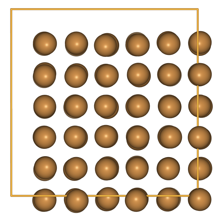
- Using the EMT potential, let us try some simulated annealing (controlled heating and cooling) of cubic Cu.
- There are three preparation steps:
- Build the structure
- Attach a calculator
- Assign initial momenta.
import ase.build
from ase.calculators.emt import EMT
from ase.md.velocitydistribution import MaxwellBoltzmannDistribution

# Set up a crystal
cu_cube = ase.build.bulk('Cu', cubic=True) * [3, 3, 3]

# Describe the interatomic interactions with the Effective Medium Theory
cu_cube.calc = EMT()

# Set the momenta corresponding to T=300K
MaxwellBoltzmannDistribution(cu_cube, temperature_K=300)
Atoms store forces, velocities and energies
row_limit = 4
print('velocities:')
print(cu_cube.get_velocities()[:row_limit])

print(f'\nkinetic energy: {cu_cube.get_kinetic_energy()}')
velocities:
[[ 0.04415792 -0.04196006 -0.02130616]
 [ 0.00674007 -0.009692    0.02499719]
 [ 0.00949497 -0.00967576  0.03271635]
 [ 0.01499601 -0.01203037 -0.02456846]]

kinetic energy: 5.209391647215017
- The initial forces should be very small due to symmetry
print('\nforces:')
print(cu_cube.get_forces()[:row_limit])
forces:
[[ 1.05748743e-14  9.68843061e-15  8.49667559e-15]
 [ 2.47839943e-14 -1.35655376e-15 -2.27769192e-15]
 [-1.81799020e-15  1.80896964e-14 -1.32012457e-15]
 [-2.18835366e-15  1.32706346e-16  1.38292156e-14]]
Create a dynamics object and then attach Atoms
- Next the dynamics object is created and the
Atomsare attached to it. - For constant-energy MD we can use the Velocity Verlet method.
- While the default distance and energy units (Angstrom and eV) in ASE are fairly friendly, the related time unit is a bit awkward so we use a unit conversion from
ase.unitsto set a timestep of 5 fs.
from ase import units
from ase.md.verlet import VelocityVerlet

dyn = VelocityVerlet(cu_cube, 5 * units.fs)
After each timestep the Atoms properties are updated
- After one timestep, we see that the velocities have changes slightly and significant forces have appeared.
dyn.run(1)


print('velocities:')
print(cu_cube.get_velocities()[:row_limit])

print('\nforces:')
print(cu_cube.get_forces()[:row_limit])
velocities:
[[ 0.04342004 -0.04111118 -0.02074165]
 [ 0.00662474 -0.01022957  0.02452406]
 [ 0.00927404 -0.00939438  0.03250037]
 [ 0.01462945 -0.01201408 -0.02386139]]

forces:
[[-0.19094268  0.21966678  0.14607907]
 [-0.02984384 -0.13910846 -0.12243429]
 [-0.05717046  0.07281418 -0.05589085]
 [-0.09485569  0.00421554  0.18297141]]
- Now we run more timesteps, printing the kinetic and potential energy every 10 steps.
from ase import Atoms

def printenergy(atoms: Atoms) -> None:
    """Function to print the potential, kinetic and total energy"""
    epot = atoms.get_potential_energy() / len(atoms)
    ekin = atoms.get_kinetic_energy() / len(atoms)
    temperature = ekin / (1.5 * units.kB)

    print(f'Energy per atom: Epot = {epot:.3f}eV  Ekin = {ekin:.3f}eV '
          f'(T={temperature:3.0f}K)  Etot = {epot+ekin:.3f}eV')

# print starting energies
printenergy(cu_cube)
# print energies as system evolves
for i in range(20):
    dyn.run(10)
    printenergy(cu_cube)
Energy per atom: Epot = 0.028eV  Ekin = 0.015eV (T=115K)  Etot = 0.043eV
Energy per atom: Epot = 0.020eV  Ekin = 0.023eV (T=175K)  Etot = 0.043eV
Energy per atom: Epot = 0.019eV  Ekin = 0.024eV (T=186K)  Etot = 0.043eV
Energy per atom: Epot = 0.012eV  Ekin = 0.031eV (T=239K)  Etot = 0.043eV
Energy per atom: Epot = 0.020eV  Ekin = 0.022eV (T=174K)  Etot = 0.043eV
Energy per atom: Epot = 0.023eV  Ekin = 0.020eV (T=151K)  Etot = 0.043eV
Energy per atom: Epot = 0.013eV  Ekin = 0.029eV (T=228K)  Etot = 0.043eV
Energy per atom: Epot = 0.022eV  Ekin = 0.021eV (T=159K)  Etot = 0.043eV
Energy per atom: Epot = 0.016eV  Ekin = 0.027eV (T=206K)  Etot = 0.043eV
Energy per atom: Epot = 0.018eV  Ekin = 0.025eV (T=194K)  Etot = 0.043eV
Energy per atom: Epot = 0.021eV  Ekin = 0.022eV (T=169K)  Etot = 0.043eV
Energy per atom: Epot = 0.019eV  Ekin = 0.023eV (T=180K)  Etot = 0.043eV
Energy per atom: Epot = 0.011eV  Ekin = 0.032eV (T=245K)  Etot = 0.043eV
Energy per atom: Epot = 0.026eV  Ekin = 0.017eV (T=128K)  Etot = 0.043eV
Energy per atom: Epot = 0.016eV  Ekin = 0.027eV (T=209K)  Etot = 0.043eV
Energy per atom: Epot = 0.019eV  Ekin = 0.024eV (T=187K)  Etot = 0.043eV
Energy per atom: Epot = 0.017eV  Ekin = 0.026eV (T=202K)  Etot = 0.043eV
Energy per atom: Epot = 0.022eV  Ekin = 0.021eV (T=160K)  Etot = 0.043eV
Energy per atom: Epot = 0.016eV  Ekin = 0.027eV (T=210K)  Etot = 0.043eV
Energy per atom: Epot = 0.018eV  Ekin = 0.024eV (T=189K)  Etot = 0.043eV
Discussion
As the system equilibrates, energy is conserved but the temperature is about half of the original setting. Why?
Solution
We started with momenta corresponding to 300K, but ideal lattice positions which correspond to 0K (in classical dynamics). The equipartition theorem states that energy should be shared equally, so half of the kinetic energy makes its way into potential energy and we are left with the momentum distribution of a lower temperature.
Attach an observer function to track properties
- It’s a bit inconvenient to write a loop that stops and starts the MD as above; instead we can attach an “observer” function.
def energy_observer():
    printenergy(cu_cube)

dyn.attach(energy_observer, interval=10)
dyn.run(100)
Exercise: RMS displacement
Use an observer to measure the average root-mean-square displacement of Cu atoms at 300K.
Hint: if the numbers seem too large, try visualising the trajectory to see what could be causing a problem.
Solution
import numpy as np
ref_atoms = ase.build.bulk('Cu', cubic=True) * [3, 3, 3]
ref_atoms.center()  # Shift centre-of-mass to the origin

def rms_observer():
    cu_cube.center()  # Remove drift, make consistent with ref
    displacements = cu_cube.positions - ref_atoms.positions
    rms_displacements = np.sqrt((displacements**2).mean(axis=0))
    print(rms_displacements)

dyn = VelocityVerlet(cu_cube, 5 * units.fs)
dyn.attach(rms_observer, interval=50)
dyn.run(400)
Attach a Trajectory object to track atom positions
- At modest temperature and under periodic boundary conditions, the atoms have not moved very far.
from ase.visualize import view

view(cu_cube, viewer='ngl')
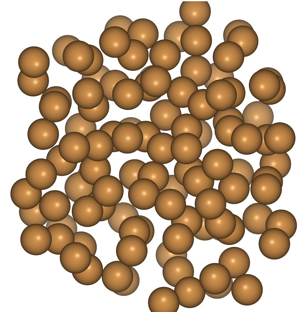
- Let’s try something more extreme:
- remove the boundary conditions
- increase the temperature
- regulate the temperature with a Langevin thermostat
- We attach a Trajectory to track atom positions
- This simulation will take a few minutes to run.
from ase.io.trajectory import Trajectory
from ase.md import Langevin

cu_lump = cu_cube.copy()
cu_lump.pbc=False
cu_lump.calc = EMT()

def energy_observer():
    printenergy(cu_lump)

dyn = Langevin(cu_lump, 5 * units.fs, friction=0.005, temperature_K=1000)
dyn.attach(energy_observer, interval=50)

# We also want to save the positions of all atoms after every 50th time step.
traj = Trajectory('cu_melt.traj', 'w', cu_lump)
dyn.attach(traj.write, interval=50)

# Now run the dynamics
dyn.run(1000)
Energy per atom: Epot = 0.458eV  Ekin = 0.025eV (T=193K)  Etot = 0.483eV
Energy per atom: Epot = 0.463eV  Ekin = 0.042eV (T=322K)  Etot = 0.504eV
Energy per atom: Epot = 0.477eV  Ekin = 0.048eV (T=372K)  Etot = 0.525eV
Energy per atom: Epot = 0.496eV  Ekin = 0.058eV (T=452K)  Etot = 0.554eV
Energy per atom: Epot = 0.493eV  Ekin = 0.070eV (T=539K)  Etot = 0.562eV
Energy per atom: Epot = 0.504eV  Ekin = 0.076eV (T=587K)  Etot = 0.580eV
Energy per atom: Epot = 0.507eV  Ekin = 0.085eV (T=661K)  Etot = 0.592eV
Energy per atom: Epot = 0.518eV  Ekin = 0.080eV (T=617K)  Etot = 0.598eV
Energy per atom: Epot = 0.511eV  Ekin = 0.095eV (T=732K)  Etot = 0.606eV
Energy per atom: Epot = 0.526eV  Ekin = 0.090eV (T=694K)  Etot = 0.616eV
Energy per atom: Epot = 0.517eV  Ekin = 0.106eV (T=821K)  Etot = 0.623eV
Energy per atom: Epot = 0.543eV  Ekin = 0.099eV (T=763K)  Etot = 0.642eV
Energy per atom: Epot = 0.551eV  Ekin = 0.094eV (T=724K)  Etot = 0.644eV
Energy per atom: Epot = 0.539eV  Ekin = 0.110eV (T=854K)  Etot = 0.650eV
Energy per atom: Epot = 0.541eV  Ekin = 0.124eV (T=959K)  Etot = 0.665eV
Energy per atom: Epot = 0.551eV  Ekin = 0.112eV (T=863K)  Etot = 0.663eV
Energy per atom: Epot = 0.568eV  Ekin = 0.099eV (T=768K)  Etot = 0.667eV
Energy per atom: Epot = 0.555eV  Ekin = 0.121eV (T=938K)  Etot = 0.676eV
Energy per atom: Epot = 0.574eV  Ekin = 0.101eV (T=782K)  Etot = 0.675eV
Energy per atom: Epot = 0.578eV  Ekin = 0.102eV (T=791K)  Etot = 0.680eV
Energy per atom: Epot = 0.590eV  Ekin = 0.101eV (T=782K)  Etot = 0.691eV
- The trajectory file lets us visualise what happened.
import ase.io

frames = ase.io.read('cu_melt.traj', index=':')
view(frames, viewer='ngl')
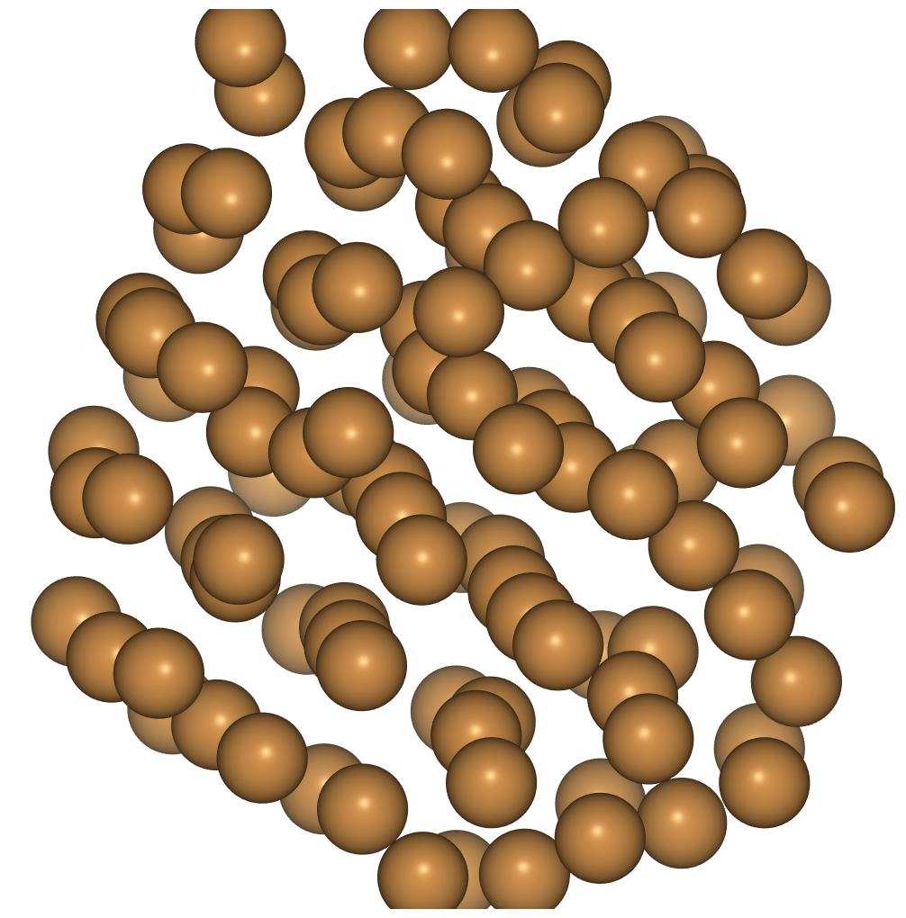
To quench, reduce the target temperature over the course of the simulation
- We see that as the temperature falls some order returns to the structure.
for temperature in range(800, 100, -50):
    dyn.set_temperature(temperature_K=temperature)
    dyn.run(100)

frames = ase.io.read('cu_melt.traj', index=':')
view(frames, viewer='ngl')
extras
in the attached archive you will find some fully worked examples of LJonesium NVE, NVT and NPT. Also a simple example of how to do a dynamic NEB optimisation for a small molecule. extra md
Key Points
Energies and forces can be used to update structures
Molecular dynamics methods are found in
ase.md
Atomsstore forces, velocities and energiesCreate a dynamics object and then attach
AtomsAfter each timestep the
Atomsproperties are updatedAttach an observer function to track properties
Attach a
Trajectoryobject to track atom positionsTo quench, reduce the target temperature over the course of the simulation