Electronic structure

Overview

Teaching: 20 min
Exercises: 20 min

Questions

• How can I use DFT to produce an electronic bandstructure?

• How can I use DFT to produce an electronic Density of States?

Objectives

Code connection

In this episode we will use Quantum Espresso to calculate the electronic structure (bandstructure and density of states) of silicon. We will analyse and plot the electronic structure using ase.dft and ase.spectrum.

We now have all the tools in place to calculate electronic structure properties

• In the previous tutorials we created Atoms objects and used the Quantum Espresso calculator to get basic properties (total energies and forces) calculated using DFT.
• We will now use this calculator to calculate and plot the band dispersion and density of states for silicon.
• This process takes four calculation steps; i) structure optimisation; ii) self-consistent calculation; iii) non-self-consistent calculation with sampling along a k-point path in reciprocal space; iv) non-self-consistent calculation with dense sampling in reciprocal space.

Note

This is not a course in DFT; for more details on the terminology used please see other sources.

The tocell() method can be used to build a FCC lattice

• The first step, as always, is to import libraries and build an Atoms object
• Here we create an FCC class instance and then convert this to a Cell object
• We will assume that the cell parameters have already been optimized.

from ase import Atoms
from ase.lattice import FCC
from ase.units import Bohr

si_fcc = Atoms(symbols='Si2',
               cell = FCC(a=10.20*Bohr).tocell(),
               scaled_positions=[(0.0, 0.0, 0.0),
                                 (0.25, 0.25, 0.25)],
               pbc=True)

Pseudopotential data are loaded from a local filepath

• Each pseudopotential-based electronic structure code is associated with a dataset describing the potentials used.
• In this case we specify the filepath to the SSSP pseudopotential library, and read this to get the kinetic energy cutoff energy values for silicon.
• We also store the pseudopotential for each species in the system of interest within a Python dictionary

Note

This is not a course in DFT; be aware that calculation parameters must be chosen with care for a given research problem.

from pathlib import Path
import json

pseudo_dir = Path.home() / 'SSSP_1.2.1_PBE_efficiency'
with open(str(pseudo_dir / 'SSSP_1.2.1_PBE_efficiency.json')) as fj:
  dj = json.load(fj) 
ecutwfc = dj['Si']['cutoff_wfc']
ecutrho = dj['Si']['cutoff_rho']

atomic_species = {'Si':dj['Si']['filename']}

Python dictionaries are used to store related calculation parameters

• There are many parameters used in a typical electronic structure calculation.
• Keywords for the Espresso class are specified as dictionaries grouping related parameters.
  • control specifies that we want to do a self-consistent calculation, a prefix to identify the calculation, the directory where the program saves the data files, and the pseudopotentials’ location;
  • system specifies the two cutoff for the FFT grid
  • electron specifies the iterative diagonalization algorithm and the convergence threshold.

control = {'calculation': "scf",
           'prefix': "si_fcc",
           'outdir': str(Path('./si_fcc/out').absolute()) ,
           'pseudo_dir': str(pseudo_dir),
           'tprnfor': True,
           'tstress': True}
system = {'ecutwfc': ecutwfc,
          'ecutrho': ecutrho}
electrons = {'diagonalization':'davidson',
             'conv_thr': 1.e-8}

EspressoProfile objects are used to hold run information

• Information for how to run QE on a particular system is stored in an EspressoProfile object.
• Here we specify two profiles
  • one where we run with 4 MPI ranks with the default parallelization
  • one where we run with 4 MPI ranks using pools parallelization

from ase.calculators.espresso import EspressoProfile

plain_argv = ['mpirun', '-np', '4', 'pw.x']
pools_argv = ['-nk', '4']
profile = EspressoProfile(plain_argv)
profile_4pools = EspressoProfile(plain_argv + pools_argv)    

Specify a directory for each calculation to avoid overwriting

• We are now ready to create an Espresso calculator for the scf calculation.
• As we are going to run few calculations we will specify a specific directory for each of them so that we don’t overwrite the input and standard-output files of the pw.x programme.
• Binary files that are read by successive calculations will be saved in the outdir input variable defined above.
• We also specify some other key information; the Monkhort-Pack mesh for kpoints, and the offset of the MP mesh.

from ase.calculators.espresso import Espresso 

scf_directory = Path('./si_fcc/scf/').absolute()

scf_calc = Espresso(directory=scf_directory,
                profile=profile,
                input_data={'control': control,
                            'system': system,
                            'electrons': electrons},
                pseudopotentials={'Si':dj['Si']['filename']},
                kpts=[8,8,8],
                koffset=[1,1,1])

• We now use the calculator to run a scf calculation for our system.

si_fcc.calc = scf_calc
props_scf = si_fcc.get_properties(['energy'])
round(props_scf['energy'],8) 

-215.69011555

Generate k-points path using the bandpath method

kpointpath = si_fcc.cell.bandpath(path='LGXWKG', density=20)
kpointpath.special_points

{'G': array([0., 0., 0.]),
 'K': array([0.375, 0.375, 0.75 ]),
 'L': array([0.5, 0.5, 0.5]),
 'U': array([0.625, 0.25 , 0.625]),
 'W': array([0.5 , 0.25, 0.75]),
 'X': array([0.5, 0. , 0.5])}

Create a new Calculator object and Atoms for the next calculation

• First we use the dictionary update method to adjust some calculation parameters.

control.update({'calculation':"bands"})
system.update({'nbnd':12})
electrons.update({'conv_thr': 1.e-6})

• Then we setup the new calculator for bands.
• We specify a new calculation directory.
• We use the profile_4pools profile, which passes the -nk 4 option to pw.x and distributes the band structure calculations over 4 autonomous pools.

bands_directory = Path('./si_fcc/bands').absolute()

bands_calc = Espresso(directory=bands_directory,
                  input_data={'control': control,
                              'system': system,
                              'electrons':electrons},
                  pseudopotentials=atomic_species, 
                  profile=profile_4pools,
                  kpts=kpointpath) 

• We copy the Atoms object to avoid overwriting results from the SCF calculation, attach the Calculator and run.

si_fcc_bands = si_fcc.copy()
si_fcc_bands.calc = bands_calc
results_bands = si_fcc_bands.get_properties(['eigenvalues']) 

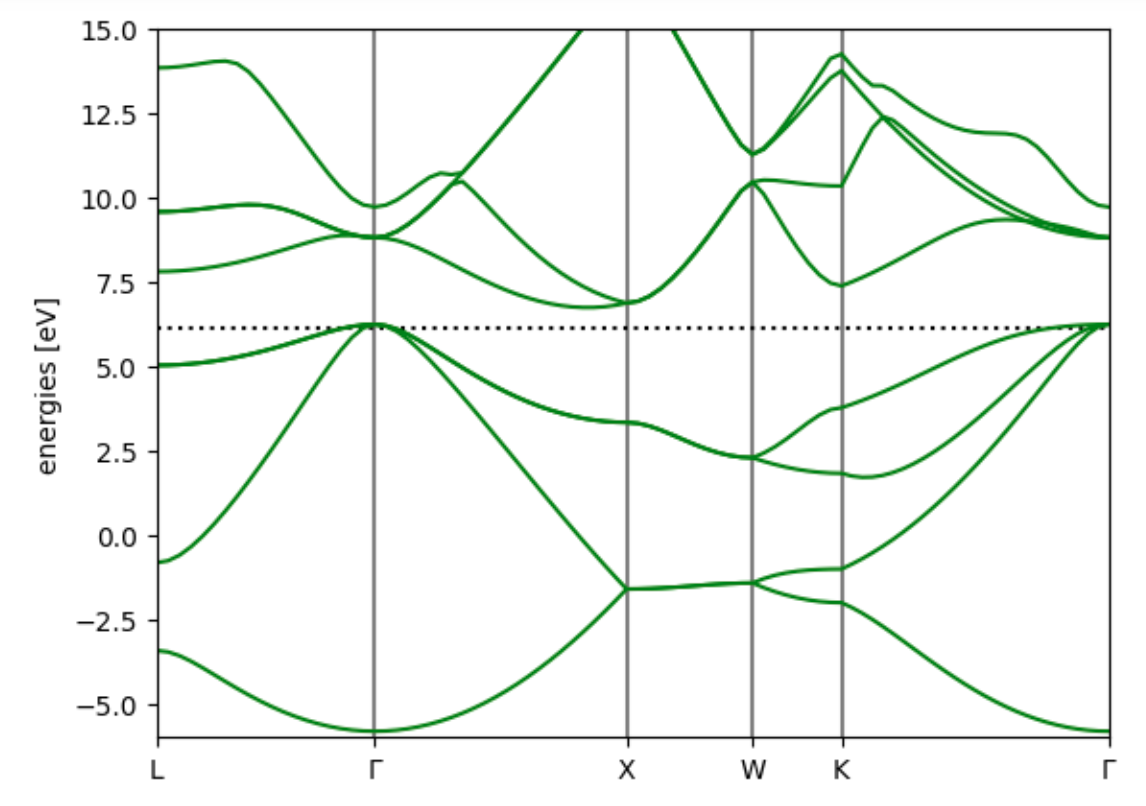
Use ase.spectrum to analyse and plot band structures

• Create a BandStructure object holding the k-point path and eigenvalues.
• Use as reference level the Fermi level that has been computed in the scf calculation.

from ase.spectrum.band_structure import BandStructure
si_fcc_band_structure = BandStructure(path=kpointpath, 
                           energies=results_bands['eigenvalues'], reference=si_fcc.calc.get_fermi_level())

• The Bandstructure object has methods for plotting and saving.

bandplot = si_fcc_band_structure.plot(emin=-6, emax=15)
bandplot.figure.savefig('band_structure_Si.png')

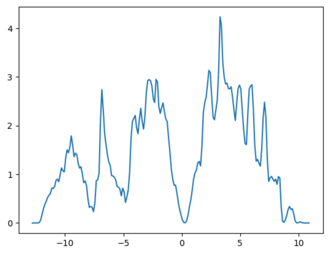
Use ase.dft to compute the Density of States

• As for the bandstructure calculation, we create a new Calculator, Atoms and calculation directory for this calculation.
• We change verbosity to ‘high’ because printout of energies in the standard output wound be suppressed for the large number of kpoints we are using.

control.update({'calculation':'nscf',
                'verbosity': 'high'})
system.update({'nbnd': 20})

nscf_directory = Path('./si_fcc/nscf').absolute() 

nscf_calc = Espresso(directory =nscf_directory,
                 profile = profile_4pools,
                 input_data={'control': control,
                             'system': system,
                             'electron': electrons}, 
                 pseudopotentials=atomic_species, 
                 kpts=[16,16,16],
                 koffset=[0,0,0]) 

si_fcc_nscf = si_fcc.copy()
si_fcc_nscf.calc = nscf_calc
nscf_results = si_fcc_nscf.get_properties(['eigenvalues'])

• We use ASE’s DOS class to compute the Density of States.

from ase.dft.dos import DOS 
from matplotlib  import pyplot as plt

dos = DOS(nscf_calc, npts = 200,width=0.2) 

• This is initialised using the Calculation object nscf_calc.
• We can then access the energies property and get_dos “getter” method needed for plotting the DOS.

energies=dos.energies
dosvals = dos.get_dos() 

plt.plot(energies, dosvals)
plt.axis([-13, 15, 0, 5])
plt.savefig('DOS_Si.png')

Key Points

• We now have all the tools in place to calculate electronic structure properties

• Use the tocell() method to build a FCC lattice

• Pseudopotential data are loaded from a local filepath

• Python dictionaries are used to store related calculation parameters

• EspressoProfile objects are used to hold run information

• Specify a directory for each calculation to avoid overwriting

• Generate k-points path using the bandpath method

• Create a new Calculator object and Atoms for the next calculation

• Use ase.spectrum to analyse and plot band structures

• Use ase.dft to compute the Density of States