Calculations in parallel

Overview

Teaching: 25 min
Exercises: 20 min

Questions

• Is it possible to run calculations in parallel using ASE?

• How can I store useful results from a script?

• How can I measure the speed-up achieved?

Objectives

• Use the GPAW Python interpreter to run a DFT calculation across multiple cores and measure the speed-up achieved

• Save the relevant data in a JSON file for further analysis

• Use the Quantum Espresso code to run a DFT calculation across multiple cores

Code connection

In this episode we perform parallel calculations with GPAW and Quantum Espresso.

To accelerate our calculation we can parallelise the code over several cores

• In the previous tutorial we performed DFT calculations with GPAW using one CPU core.
• This approach will be too slow for many useful calculations.

Parallel programming systems

There are several schemes for parallelising code. The two most common are MPI and OpenMP, with the optimum choice dependent on both the code and the hardware being used (for example, memory or CPU architecture, number of cores per node, network speed). Increasingly, electronic structure codes enable a hybrid of both approaches.

• To split our code over several MPI processes we will use a special GPAW Python interpreter.
• We will use this to run a script file named “kpts_parallel.py”. This is very similar to the code we used before, except we will:
  • use the parallel keyword to switch on k-point parallelisation.
  • write a dictionary of the results to a json file.

parprint and paropen are provided in ASE as an alternative to print and open

• Commands such as print or open can cause data corruption when multiple processes try to write to the same file.
• parprint and paropen are provided in ASE to handle these common cases
• For other scenarios it may be necessary to use logic with ase.parallel.world. For more information see the relevant GPAW docs and ASE docs

Do not run this code in your notebook!

The next code block should go into a new script file named “kpts_parallel.py”

from gpaw import GPAW, PW

import ase.build
from ase.parallel import parprint, world, paropen
from ase.utils.timing import Timer
import json

atoms = ase.build.bulk('Cu')

timer = Timer()
energies, times, nkpts = [], [], []

for k in range(3, 9):

    atoms.calc = GPAW(mode=PW(400), xc='PBE',
                      kpts={'size': [k, k, k],
                            'gamma': False},
                      txt='kpts_parallel.txt',
                      parallel={'kpt': True})
    timer.start(str(k))
    energy = atoms.get_potential_energy()
    timer.stop(str(k))
    energies.append(energy)
    times.append(timer.get_time(str(k)))
    nkpts.append(len(atoms.calc.get_ibz_k_points()))

with paropen('parallel_results.json', 'w') as file:
    json.dump({'energies': energies,
               'times': times,
               'nkpts': nkpts},
              file)

• Now we are ready to run the script from the command-line.
• The -P option sets the number of MPI tasks, in this case 4.
• The parallel Python process essentially runs 4 copies of the script. (TODO: check this?)

gpaw -P 4 python kpts_parallel.py

• Finally, we can plot the results back in our main Python session.
• (This assumes the energies and times variables are still available from the previous tutorial. If not, you will need to run the serial example again!)
• The new energies and times are read from a JSON file. This is a useful format for saving and loading simple Python dictionary data, and is interoperable with many programming languages and software tools.

import json

with open('parallel_results.json', 'r') as file:
    parallel_data = json.load(file)

fig, axes = plt.subplots(nrows=3, sharex=True)

axes[0].plot(nkpts, energies, 'o-', label='serial')
axes[0].plot(parallel_data['nkpts'], parallel_data['energies'], 'o', label='parallel')
axes[0].set_ylabel('energy / eV')
axes[0].legend()

axes[1].plot(nkpts, times, 'o-', label='serial')
axes[1].plot(parallel_data['nkpts'], parallel_data['times'], 'o-', label='parallel')
axes[1].set_ylabel('Calculation time / s')
axes[1].legend()
axes[1].set_ylim([0, None])

axes[2].plot(nkpts, np.asarray(times) / parallel_data['times'], label='4 cores')
axes[2].set_ylabel('Speed-up factor')
axes[2].set_xlabel('number of k-points')

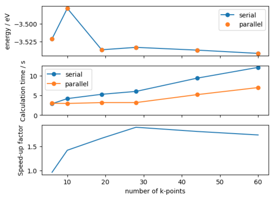
• We find that the parallel calculation is faster, but not 4 times faster.
• This is because it is not possible to parallelise all parts of the code.

Quantum Espresso can also be used for parallel programming with MPI

• Unlike GPAW, we are going to call the program with MPI from within our regular Python interpreter.
• We define the mpi command when instantiating the calculator: the command might need to be tweaked for different machines with different parallel environments.
• This information is captured in a “Profile” object.

Getting the data

We will use the SSSP-efficiency pseudopotential set. To download these from a Jupyter Notebook run the following in a cell:

%%bash

mkdir SSSP_1.2.1_PBE_efficiency

wget -q https://archive.materialscloud.org/record/file?record_id=1680\&filename=SSSP_1.2.1_PBE_efficiency.tar.gz -O SSSP-efficiency.tar.gz

wget -q https://archive.materialscloud.org/record/file?filename=SSSP_1.2.1_PBE_efficiency.json\&record_id=1732 -O SSSP_1.2.1_PBE_efficiency.json

tar -zxvf SSSP-efficiency.tar.gz -C ./SSSP_1.2.1_PBE_efficiency

mv SSSP_1.2.1_PBE_efficiency.json ./SSSP_1.2.1_PBE_efficiency/

Note

Profiles are a fairly new ASE feature and not yet used by all such Calculators. An alternative way to manage these commands is by setting environment variables, e.g. ASE_ESPRESSO_COMMAND. Check the docs for each calculator to see what is currently implemented.

from ase.calculators.espresso import Espresso, EspressoProfile

profile = EspressoProfile(['mpirun', 'pw.x'])

Each Calculator has its own keywords to match the input syntax of the corresponding software code

• You can see below that the keywords for the Espresso() class are different to those from the GPAW() class.
• This is because each software code requires different input parameters.
• For QE, the content of input_data contains the parameters for the calculation input file.

pseudo_dir = Path.home() / 'SSSP-1.2.1_PBE_efficiency'

calc = Espresso(profile=profile,
                pseudo_dir=pseudo_dir,
                kpts=(3, 3, 3),
                input_data={'control':  {'tprnfor': True,
                                         'tstress': True},
                            'system': {'ecutwfc': 50.}},
                pseudopotentials={'Si': 'Si.pbe-n-rrkjus_psl.1.0.0.UPF'})

Once we have setup the calculator we use the same three step process to retrieve a property

• The difficult part is setting up the calculator!
• Once setup is complete, we can get a total energy using the same three-step process.

atoms = ase.build.bulk('Si')
atoms.calc = calc
atoms.get_potential_energy()

-310.1328387367529

• As this is a file-based calculator we can inspect the input file automatically generated, espresso.in, and confirm that there is a straightforward relationship between the keys used for the input_data parameter and the espresso input.

cat espresso.in

Exercise: Basis set convergence

As well as k-point sampling, basis-set convergence should be checked with respect to meaningful properties. Check the convergence of the atomisation energy of Si with respect to the Espresso parameter ecutwfc - the basis set cutoff energy in Ry. What cutoff energy is needed for a convergence level of 1 meV?

Hint: to calculate the atomisation energy, you will need to compare the energy of the solid to a single atom in a large cell.

Hint: you will need to calculate this property at several cutoff energies. Use Python functions and iteration constructs to avoid too much repetition.

Key Points

• To accelerate our calculation we can parallelise the code over several cores

• parprint and paropen are provided in ASE as an alternative to print and open

• Quantum Espresso can also be used for parallel programming with MPI

• Each Calculator has its own keywords to match the input syntax of the corresponding software code

• Once we have setup the calculator we use the same three step process to retrieve a property