Local optimisation

Overview

Teaching: 20 min
Exercises: 30 min

Questions

How can I find kinetically stable structures?

Is it possible to apply constraints to my system?

How can I optimise other degrees of freedom beyond atom positions?

Can I generate amorphous structures using ASE?

Objectives

Perform geometry optimization using MOPAC

Perform molecular dynamics and geometry optimisation using a machine learned potential

Apply constraints to an optimisation routine

Code connection

In this episode we will use the ase.optimize module to perform geometry optimisation, and ase.constraints to constrain or optimise various degrees of freedom.

To minimise energy and forces we typically use an optimisation algorithm

With a zero temperature thermostat we would eventually expect the structure to reach some local minimum energy in the potential-energy surface.
Generally it is more efficient to achieve this by a dedicated “geometry optimisation” algorithm that seeks to minimise energy and forces.
Let’s grab a molecular structure and apply a semi-empirical potential to calculate forces.

from ase.calculators.mopac import MOPAC

atoms = ase.build.molecule('CH3CH2OH')
atoms.calc = MOPAC()
atoms.get_forces()

          MOPAC Job: "mopac.mop" ended normally on Apr 17, 2023, at 11:15.

array([[ 0.05314722, -0.14217078,  0.        ],
       [ 0.08516519,  0.2916233 ,  0.        ],
       [ 0.46667555,  0.31685049,  0.        ],
       [-0.30313837, -0.04753196,  0.        ],
       [-0.29917533,  0.04623103,  0.23729349],
       [-0.2992056 ,  0.04519975, -0.23729349],
       [ 0.11622196, -0.06459161,  0.        ],
       [ 0.09013888, -0.22333767,  0.08025091],
       [ 0.09017054, -0.22227256, -0.08025091]])

There are a range of algorthms in the `ase.optimize` module

We can see from the forces that this potential does not quite agree with the structure from the G2 database.
For further calculations using MOPAC we need to find the local minimum.
ASE provides a range of algorthms in the ase.optimize module.
There are three preparation steps:
- Build the Atoms structure
- Attach a Calculator object
- Instantiate the optimisation object with the Atoms object

from ase.optimize import GPMin
# To avoid that "ended normally" message on every step, we
# tweak the command a bit
atoms = ase.build.molecule('CH3CH2OH')
atoms.calc = MOPAC(command='mopac PREFIX.mop 1> /dev/null')
opt = GPMin(atoms)

When we run the optimisation the original Atoms object updates its positions.

opt.run(fmax=1e-3)
atoms.get_forces()

       Step     Time          Energy          fmax
GPMin:    0 11:15:28       -2.385274         0.564075
GPMin:    1 11:15:28       -2.392905         1.033572
GPMin:    2 11:15:28       -2.403956         0.742120
GPMin:    3 11:15:28       -2.420694         0.221260
GPMin:    4 11:15:28       -2.421733         0.151170
GPMin:    5 11:15:28       -2.422788         0.015994
GPMin:    6 11:15:28       -2.422797         0.010651
GPMin:    7 11:15:28       -2.422799         0.006327
GPMin:    8 11:15:28       -2.422801         0.003863
GPMin:    9 11:15:28       -2.422801         0.000485

array([[ 7.17242279e-05,  1.52121276e-04, -2.75015147e-04],
       [ 2.59490798e-04,  9.01106079e-05,  4.03286166e-06],
       [-4.31949839e-04, -1.41150158e-04,  1.70377564e-04],
       [ 1.22850506e-04, -3.39324113e-04,  3.42142780e-05],
       [-6.14902993e-05,  4.04153448e-05, -5.03023605e-05],
       [-1.96786304e-04, -1.73499780e-04, -1.32824250e-04],
       [ 1.40066056e-05,  1.05244680e-04,  2.27704910e-04],
       [-3.03548727e-05, -6.07097455e-05,  8.32590795e-06],
       [ 2.52552541e-04,  3.26878615e-04,  1.34862363e-05]])

Exercise: Comparing optimisers

Compare the results and performance of QuasiNewton, FIRE and GPMin optimizers for a few small organic molecules.

We can apply constraints to the `Atoms` object before optimisation

We don’t always want to optimize every degree of freedom; perhaps we can assume some region is rigid, or we are using a forcefield that fixes some bond length.
In ASE this is achieved by applying constraints to the Atoms object before optimisation.
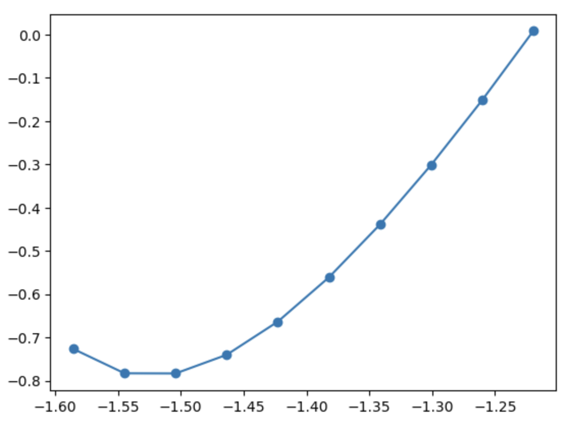
Suppose we want to explore the effect of stretching the C-C bond in ethane, while allowing the hydrogen atoms to relax to their local minimum at each configuration.
The steps are largely the same as in the previous calculation
- Build the Atoms structure (build_stretched_ethane)
- Apply a constraint (build_stretched_ethane)
- Attach a calculator (get_optimised_energy)
- Create an optimisation object (get_optimised_energy)
- Run the optimisation routine (get_optimised_energy)
Python list comprehension is used to repeat the process for various C-C bond lengths

from ase.constraints import FixAtoms
import numpy as np

ethane = ase.build.molecule('C2H6')
g2_c_c = ethane.positions[1, 2] - ethane.positions[0, 2]
constraint = FixAtoms(mask=(atoms.symbols == 'C'))

def build_stretched_ethane(d: float = g2_c_c) -> Atoms:
    shift = (d - g2_c_c) / 2
    ethane = ase.build.molecule('C2H6')
    ethane.positions[[0, 2, 3, 4]] += [0, 0, shift]
    ethane.positions[[1, 5, 6, 7]] -= [0, 0, shift]
    ethane.set_constraint(constraint)
    return ethane

def get_optimised_energy(atoms: Atoms) -> float:
    # Redirect STDOUT to avoid annoying message on every step
    atoms.calc = MOPAC(command='mopac PREFIX.mop 1> /dev/null')
    opt = GPMin(atoms)
    opt.run(fmax=1e-3)
    return atoms.get_potential_energy()

lengths = np.linspace(0.8, 1.04, 10) * g2_c_c
energies = [get_optimised_energy(build_stretched_ethane(d)) for d in lengths]

Step     Time          Energy          fmax
GPMin:    0 11:15:29        0.208544         0.693187
GPMin:    1 11:15:29        0.010296         0.115406
GPMin:    2 11:15:29        0.008034         0.024697
GPMin:    3 11:15:29        0.007877         0.011408
GPMin:    4 11:15:29        0.007868         0.001131
GPMin:    5 11:15:29        0.007871         0.000784
       Step     Time          Energy          fmax
GPMin:    0 11:15:29        0.004891         0.621748
GPMin:    1 11:15:29       -0.148598         0.110453
GPMin:    2 11:15:29       -0.151673         0.029460
GPMin:    3 11:15:29       -0.151831         0.010914
GPMin:    4 11:15:29       -0.151840         0.001365
GPMin:    5 11:15:30       -0.151837         0.000968
       Step     Time          Energy          fmax
GPMin:    0 11:15:30       -0.185557         0.542410
GPMin:    1 11:15:30       -0.297151         0.110753
GPMin:    2 11:15:30       -0.301405         0.033660
GPMin:    3 11:15:30       -0.301558         0.011636
GPMin:    4 11:15:30       -0.301564         0.006232
GPMin:    5 11:15:30       -0.301566         0.001605
GPMin:    6 11:15:30       -0.301564         0.000377
       Step     Time          Energy          fmax
GPMin:    0 11:15:30       -0.359554         0.454383
GPMin:    1 11:15:30       -0.433351         0.115860
GPMin:    2 11:15:30       -0.438910         0.036632
GPMin:    3 11:15:30       -0.439056         0.011921
GPMin:    4 11:15:30       -0.439063         0.001158
GPMin:    5 11:15:30       -0.439061         0.000215
       Step     Time          Energy          fmax
GPMin:    0 11:15:30       -0.512800         0.356939
GPMin:    1 11:15:30       -0.554601         0.120804
GPMin:    2 11:15:30       -0.561024         0.037269
GPMin:    3 11:15:30       -0.561161         0.009839
GPMin:    4 11:15:30       -0.561165         0.001118
GPMin:    5 11:15:31       -0.561165         0.000591
       Step     Time          Energy          fmax
GPMin:    0 11:15:31       -0.639633         0.249621
GPMin:    1 11:15:31       -0.657675         0.114301
GPMin:    2 11:15:31       -0.663367         0.034829
GPMin:    3 11:15:31       -0.663479         0.006902
GPMin:    4 11:15:31       -0.663481         0.001379
GPMin:    5 11:15:31       -0.663481         0.000663
       Step     Time          Energy          fmax
GPMin:    0 11:15:31       -0.732713         0.133629
GPMin:    1 11:15:31       -0.738455         0.063419
GPMin:    2 11:15:31       -0.740055         0.018883
GPMin:    3 11:15:31       -0.740080         0.007060
GPMin:    4 11:15:31       -0.740082         0.000661
       Step     Time          Energy          fmax
GPMin:    0 11:15:31       -0.782718         0.048157
GPMin:    1 11:15:31       -0.783098         0.022657
GPMin:    2 11:15:31       -0.783185         0.003206
GPMin:    3 11:15:31       -0.783185         0.000318
       Step     Time          Energy          fmax
GPMin:    0 11:15:31       -0.778047         0.160836
GPMin:    1 11:15:31       -0.782210         0.063283
GPMin:    2 11:15:31       -0.782847         0.007287
GPMin:    3 11:15:31       -0.782853         0.000394
       Step     Time          Energy          fmax
GPMin:    0 11:15:31       -0.704544         0.316270
GPMin:    1 11:15:31       -0.706982         0.214952
GPMin:    2 11:15:31       -0.726086         0.073858
GPMin:    3 11:15:31       -0.726699         0.006312
GPMin:    4 11:15:31       -0.726703         0.001655
GPMin:    5 11:15:31       -0.726703         0.000322

%matplotlib inline
import matplotlib.pyplot as plt
plt.plot(lengths, energies, 'o-')

energy as a function of C-C bondlength

Filters can be used to optimise other degrees of freedom

By default the geometry optimization only considers the atomic positions.
To present other degrees of freedom, ASE includes “filters” that present them to the optimizer.
Suppose we want to find the minimum-energy Si lattice parameters for a GAP machine-learned potential.
First lets set up the Atoms object and attach the calculator

Note

More information on the Quippy Potential object for GAP can be found in the External Calculators episode.

from ase.constraints import StrainFilter

from pathlib import Path
from quippy.potential import Potential

gap = Potential(param_filename=str(Path.cwd() / 'Si_PRX_GAP/gp_iter6_sparse9k.xml'))
si = ase.build.bulk('Si', cubic=True)
si.calc = gap

Filters place different information into the `Atoms` properties interface

The filter presents a similar interface to Atoms, but “cheats” and puts different information into the positions data.
In this case position is the a strain relative to the initial unit cell, and stresses are remapped to forces.

si_strain = StrainFilter(si)
print(si_strain.get_positions())
print(si_strain.get_forces())

array([[0., 0., 0.],
       [0., 0., 0.]])

array([[ 1.55837119e+00,  1.55837119e+00,  1.55837119e+00],
       [ 7.06032455e-16, -6.41847686e-17, -8.67361738e-18]])

To get a Si lattice with very low stress we run the optimisation with the filter as the Atoms object:

from ase.optimize import QuasiNewton
opt = QuasiNewton(si_strain)
opt.run(fmax=1e-4)

print(f"Lattice parameter: {si.cell.lengths()[0]}")
print("Residual stress:")
print(si.get_stress())

                Step[ FC]     Time          Energy          fmax
*Force-consistent energies used in optimization.
BFGSLineSearch:    0[  0] 11:15:35    -1305.407858*       2.6992
BFGSLineSearch:    1[  2] 11:15:36    -1305.420818*       0.3445
BFGSLineSearch:    2[  3] 11:15:36    -1305.421038*       0.0080
BFGSLineSearch:    3[  4] 11:15:36    -1305.421038*       0.0000

Lattice parameter: 5.460914996056226
Residual stress:
[-8.62027513e-08 -8.62027472e-08 -8.62027630e-08 -2.58637937e-15
 -6.90550987e-15 -4.46639070e-15]

We can optimise the lattice vectors and positions at the same time using a UnitCellFilter or the more sophisticated ExpCellFilter.

MD and geometry optimization can be combined to find glassy local-minimum phases

Let’s generate an amorphous Si cell by i) stretching a supercell and running a few steps of high-temperature MD; ii) performing a local optimisation to find a glassy local-minimum phase.
Step i) is a similar process to the Cu calculation in the previous episode, but now we are keeping the periodic boundary and using a machine-learned potential.
It should take a few minutes to run.

def printenergy(atoms: Atoms) -> None:
    """Function to print the potential, kinetic and total energy"""
    epot = atoms.get_potential_energy() / len(atoms)
    ekin = atoms.get_kinetic_energy() / len(atoms)
    temperature = ekin / (1.5 * units.kB)
    
    print(f'Energy per atom: Epot = {epot:.3f}eV  Ekin = {ekin:.3f}eV '
          f'(T={temperature:3.0f}K)  Etot = {epot+ekin:.3f}eV')

def energy_observer():
    printenergy(si)

si = ase.build.bulk('Si', cubic=True) * [2, 2, 2]
si.set_cell(si.cell * 1.2, scale_atoms=True)
si.calc = gap
si.calc.name = 'Si melt'

MaxwellBoltzmannDistribution(si, temperature_K=3000)
dyn = Langevin(si, 5 * ase.units.fs, friction=0.002, temperature_K=3000)
dyn.attach(energy_observer, interval=20)
traj = Trajectory('si_melt.traj', 'w', si)
dyn.attach(traj.write, interval=20)
dyn.run(400)

Energy per atom: Epot = 0.457eV  Ekin = 0.055eV (T=423K)  Etot = 0.512eV
Energy per atom: Epot = 0.457eV  Ekin = 0.055eV (T=423K)  Etot = 0.512eV
Energy per atom: Epot = 0.457eV  Ekin = 0.055eV (T=423K)  Etot = 0.512eV
Energy per atom: Epot = 0.457eV  Ekin = 0.055eV (T=423K)  Etot = 0.512eV
Energy per atom: Epot = 0.457eV  Ekin = 0.055eV (T=423K)  Etot = 0.512eV
Energy per atom: Epot = 0.457eV  Ekin = 0.055eV (T=423K)  Etot = 0.512eV
Energy per atom: Epot = 0.457eV  Ekin = 0.055eV (T=423K)  Etot = 0.512eV
Energy per atom: Epot = 0.457eV  Ekin = 0.055eV (T=423K)  Etot = 0.512eV
Energy per atom: Epot = 0.457eV  Ekin = 0.055eV (T=423K)  Etot = 0.512eV
Energy per atom: Epot = 0.457eV  Ekin = 0.055eV (T=423K)  Etot = 0.512eV
Energy per atom: Epot = 0.457eV  Ekin = 0.055eV (T=423K)  Etot = 0.512eV
Energy per atom: Epot = 0.457eV  Ekin = 0.055eV (T=423K)  Etot = 0.512eV
Energy per atom: Epot = 0.457eV  Ekin = 0.055eV (T=423K)  Etot = 0.512eV
Energy per atom: Epot = 0.457eV  Ekin = 0.055eV (T=423K)  Etot = 0.512eV
Energy per atom: Epot = 0.457eV  Ekin = 0.055eV (T=423K)  Etot = 0.512eV
Energy per atom: Epot = 0.457eV  Ekin = 0.055eV (T=423K)  Etot = 0.512eV
Energy per atom: Epot = 0.457eV  Ekin = 0.055eV (T=423K)  Etot = 0.512eV
Energy per atom: Epot = 0.457eV  Ekin = 0.055eV (T=423K)  Etot = 0.512eV
Energy per atom: Epot = 0.457eV  Ekin = 0.055eV (T=423K)  Etot = 0.512eV
Energy per atom: Epot = 0.457eV  Ekin = 0.055eV (T=423K)  Etot = 0.512eV
Energy per atom: Epot = 0.457eV  Ekin = 0.055eV (T=423K)  Etot = 0.512eV

We now optimise lattice vectors and atom positions using the ExpCellFilter.

Discussion

Note that the trajectory writer is directed to the original Si Atoms object, not the filtered version. Why?.

from ase.constraints import ExpCellFilter
si_expcell = ExpCellFilter(si)
opt = QuasiNewton(si_expcell)
traj = Trajectory('si_glass.traj', 'w', si)
opt.attach(traj)
opt.run(fmax=1e-3)

Step[ FC]     Time          Energy          fmax
*Force-consistent energies used in optimization.
BFGSLineSearch:    0[  0] 11:23:00   -10438.560479*       0.0082
BFGSLineSearch:    1[  2] 11:23:02   -10438.560479*       0.0083
BFGSLineSearch:    2[  4] 11:23:05   -10438.560479*       0.0021
BFGSLineSearch:    3[  6] 11:23:07   -10438.560479*       0.0130
BFGSLineSearch:    4[  8] 11:23:10   -10438.560479*       0.0008

We can confirm that the forces and stresses are low, so we should be in a local minimum.

print("Max force:")
print(np.linalg.norm(si.get_forces(), axis=1).max())

print("Stress:")
print(si.get_stress())

Max force:
0.000764832698961055
Stress:
[ 1.17734167e-07  5.24076825e-08 -1.70158721e-07 -1.69164613e-08
 -3.43769568e-08 -9.34363441e-09]

Exercise: Comparing crystal and amorphous Si

Compare the energy and lattice vectors of the amorphous and crystalline Si.

Exercise: Fixing the symmetry

A very useful constraint is the FixSymmetry class. Find a geometry file for a high-symmetry crystal structure. With a Calculator of your choice, perform a geometry optimization of the lattice vectors and atomic positions while fixing the symmetry. If compute power allows, you may choose to use DFT. If using Quantum Espresso, you may find it helpful to look at the SocketIOCalculator setup in the extra content section.

Key Points

To minimise energy and forces we typically use an optimisation algorithm

There are a range of algorthms in the ase.optimize module

We can apply constraints to the Atoms object before optimisation

Filters can be used to optimise other degrees of freedom

Filters place different information into the Atoms properties interface

MD and geometry optimization can be combined to find glassy local-minimum phases

previous episode

Local optimisation

next episode

Local optimisation

Overview

Code connection

To minimise energy and forces we typically use an optimisation algorithm

There are a range of algorthms in the `ase.optimize` module

Exercise: Comparing optimisers

We can apply constraints to the `Atoms` object before optimisation

Filters can be used to optimise other degrees of freedom

Note

Filters place different information into the `Atoms` properties interface

MD and geometry optimization can be combined to find glassy local-minimum phases

Discussion

Exercise: Comparing crystal and amorphous Si

Exercise: Fixing the symmetry

Key Points

previous episode

next episode

previous episode

Local optimisation

next episode

Local optimisation

Overview

Code connection

To minimise energy and forces we typically use an optimisation algorithm

There are a range of algorthms in the ase.optimize module

Exercise: Comparing optimisers

We can apply constraints to the Atoms object before optimisation

Filters can be used to optimise other degrees of freedom

Note

Filters place different information into the Atoms properties interface

MD and geometry optimization can be combined to find glassy local-minimum phases

Discussion

Exercise: Comparing crystal and amorphous Si

Exercise: Fixing the symmetry

Key Points

previous episode

next episode

There are a range of algorthms in the `ase.optimize` module

We can apply constraints to the `Atoms` object before optimisation

Filters place different information into the `Atoms` properties interface