Built-in calculators

Overview

Teaching: 20 min
Exercises: 25 min

Questions

• How can I calculate standard properties using a built-in calculator?

• How can I fit simple models to my calculations?

• What is the best way to store and share property data?

Objectives

• Calculate properties using a built-in Calculator object

• Identify the optimum bonding length for a simple metallic system

Code connection

In this episode we explore the ase.calculatorse.emt module and ase.calculatorse.lj module, both of which provide built-in tools for calculating standard properties (energy, forces and stress) from a set of atomic positions.

Atoms objects can calculate properties using an attached “Calculator”

• In ASE, Atoms objects can try to calculate or fetch properties using an attached Calculator.
• In this tutorial we will make tour of a variety of Calculators, highlighting some of the differences between them.
• A master list of the available Calculators can be found here.

Properties of metal alloy systems can be calculated using Effective Medium Theory

• Much of the ASE documentation and tutorials makes use of the built-in “EMT” calculator
• This is because it is convenient and “fast enough”
• EMT implements the Effective Medium Theory potential for Ni, Cu, Pd, Ag, Pt and Au.
• Some other elements are included “for fun”, but really this is a method for alloys of those metals.

Warning

If you want to do a real application using EMT, you should use the much more efficient implementation in the ASAP calculator.

Calculators can calculate properties in three easy steps

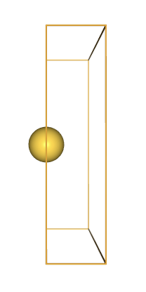
• EMT can be used to calculate, for example, the energy of an infinite gold wire.
• The first step is to create an Atoms object describing a gold wire which is infinite in the x-direction.

Python tip

You may not recognise or understand the syntax used in the function definition, for example spacing: float = 2.5. These are optional Type Hints, which were added in Python 3.5 (2015) and are becoming more widely-used as support is dropped for older versions.

from ase import Atoms
from ase.calculators.emt import EMT
from ase.visualize import view

def make_wire(spacing: float = 2.5,
              box_size: float = 10.0) -> Atoms:

    wire = Atoms('Au',
                 positions=[[0., box_size / 2, box_size / 2]],
                 cell=[spacing, box_size, box_size],
                 pbc=[True, False, False])
    return wire

atoms = make_wire()
view(atoms, viewer='ngl')

• The second step is to attach the calculator of choice, in this case EMT()

atoms.calc = EMT()

• The third and final step is to call a “getter” method for the property of choice, in this case the potential energy.

energy = atoms.get_potential_energy()
print(f"Energy: {energy} eV")

Energy: 0.9910548478768826 eV

Discussion

Why did we need the parentheses () in the line atoms.calc = EMT()?

Scientific Python libraries allow us to fit models to our calculations

• We can use the workflow above to investigate how energy varies with the atom spacing and fit a model.
• First we wrap the workflow up within a single function which returns the energy for a given atom spacing.

Python tip

if you need to apply a function to each element of some data, map can provide an elegant alternative to for-loops and list comprehensions!

import numpy as np
distances = np.linspace(2., 3., 21)

def get_energy(spacing: float) -> float:
    atoms = make_wire(spacing=spacing)
    atoms.calc = EMT()
    return atoms.get_potential_energy()

energies = list(map(get_energy, distances))

• Second we use Numpy to fit a polynomial to the generated data

from numpy.polynomial import Polynomial
fit = Polynomial.fit(distances, energies, 3)

• Finally we use Matplotlib to visualise the data and fit

IPython Magics

%matplotlib inline turns on “inline plotting”, where plots will appear in your notebook rather than as a separate pop-out window. This is our first example of an IPython magic command. You will see more examples later in the tutorial.

%matplotlib inline

import matplotlib.pyplot as plt
fig, ax = plt.subplots()
x = np.linspace(2., 3., 500)

_ = ax.plot(distances, energies, 'o', label='calculated')
_ = ax.plot(x, fit(x), '-', label='cubic')
_ = ax.legend()
_ = ax.set_xlabel('Spacing / Å')
_ = ax.set_ylabel('Energy / eV')

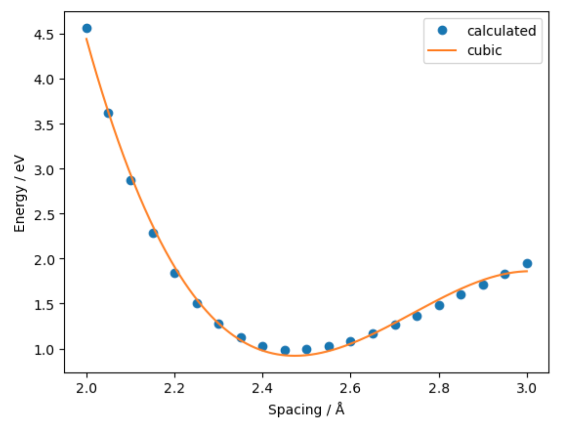
Exercise: Equation of State for bulk gold

The plot above resembles the Equation-of-State (EOS) curve for a solid. Using a similar workflow and the EquationOfState class, fit an equation of state to bulk gold and obtain an equilibrium volume.

The EMT Calculator can also be used to obtain forces and unit cell stress

print("Forces: ")
print(atoms.get_forces())

print("Stress: ")
print(atoms.get_stress())

Forces: 
[[0. 0. 0.]]
Stress: 
[ 0.00396458 -0.         -0.         -0.         -0.         -0.        ]

Discussion

Why are the forces exactly zero for this system?

• We can check which properties are implemented by a particular calculator by inspecting the implemented properties attribute:

print(EMT.implemented_properties)

['energy', 'free_energy', 'energies', 'forces', 'stress', 'magmom', 'magmoms']

Discussion

Why do we not need to include parenthesis () here? Do we expect EMT().implemented_properties to work as well as EMT.implemented_properties?

Where possible request a standalone set of property data

• It is sometimes convenient to have properties attached to a particular Calculator object.
• For example, forces are used heavily by dynamics and optimizer routines, as we will see in the next tutorial.
• However for Open Science purposes it is easier to store and share data that is not connected to a Calculator. This is because Calculators might depend on a particular machine environment, memory state or software license.
• We can request a standalone set of property data with get_properties.

properties = atoms.get_properties(['energy', 'forces', 'stress'])
print(properties)

(Properties({'energy': 0.9910548478768826, 'natoms': 1, 'energies': array([0.99105485]), 'free_energy': 0.9910548478768826, 'forces': array([[0., 0., 0.]]), 'stress': array([ 0.00396458, -0.        , -0.        , -0.        , -0.        ,
       -0.        ])})

• Importantly, this will not change even if the Atoms object is modified and properties are recalculated.

Warning

This is a new feature and does not yet work well for all calculators.

The Lennard-Jones potential can be used to model the interaction between two non-bonding atoms or molecules

• The classic Lennard-Jones potential is implemented in ase.calculators.lj.
• You can set the ε and σ parameters in the Calculator constructor:

from ase.calculators.lj import LennardJones

l = 4.1
atoms = Atoms('Xe2',
              positions=[[0., 0., -l / 2],
                         [0., 0., l / 2]],
              pbc=False)
atoms.calc = LennardJones(sigma=(4.1 / 2**(1/6)))

atoms.get_forces()

array([[ 0.00000000e+00,  0.00000000e+00, -6.49886649e-16],
       [ 0.00000000e+00,  0.00000000e+00,  6.49886649e-16]])

Discussion

Why are the forces so low at this geometry?

Exercise: Lennard-Jones binding curve

Try varying the distance between the atoms. Can you reproduce the classic plot of a Lennard-Jones binding curve?

Key Points

• Atoms objects can calculate properties using an attached Calculator

• Properties of metal alloy systems can be calculated using Effective Medium Theory

• Calculators can calculate properties in three easy steps

• Scientific Python libraries allow us to fit models to our calculations

• The EMT Calculator can also be used to obtain forces and unit cell stress

• Where possible request a standalone set of property data

• The Lennard-Jones potential can be used to model the interaction between two non-bonding atoms or molecules